
[ad_1]
Python has turn into a preferred language amongst merchants and monetary analysts because of its versatility and in depth information evaluation and visualization libraries. One highly effective utility of Python within the buying and selling world is backtesting methods, permitting merchants to judge the efficiency of their buying and selling concepts utilizing historic information. Immediately we present you a Python Bollinger Band buying and selling technique.
Bollinger bands are a broadly technical indicator that helps determine potential worth reversals and volatility in monetary markets. John Bollinger developed them and are quite simple and intuitive to make use of. We present a whole buying and selling technique with buying and selling guidelines and outcomes.
This text will stroll by the important steps of backtesting a Bollinger Band buying and selling technique. We’ll begin by explaining the foundations and logic behind the technique, discussing easy methods to arrange the required information, and eventually, offering a Python code implementation for backtesting.
Associated studying:
Python-related assets
Now we have written many articles about Python, and also you would possibly discover these attention-grabbing:
Downloading the information
To be able to backtest a buying and selling technique, we first must obtain the historic information of the shares or ETFs. In Python, the yfinance library offers a handy and environment friendly technique of engaging in this process. If you wish to study extra concerning the yfinance library see this publish:
- Best Python Libraries For Algorithmic Trading (Examples)
- How To Download Data For Your Trading Strategy From Yahoo!Finance With Python
- How To Build A Trading Strategy From FRED Data In Python (Strategy, Backtest, Rules)
- Python and RSI Trading Strategy (Backtest, Rules, Code, Setup)
- Python and Trend Following Trading Strategy (Backtest, Rules, Code, Setup)
- Python and Momentum Trading Strategy (Backtest, Rules, Code, Setup)
- Python and MACD Trading Strategy: Backtest, Rules, Code, Setup, Performance
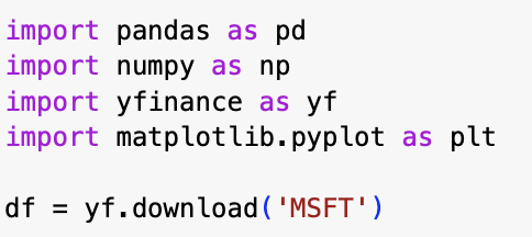
First, we have to import the libraries. We might be utilizing pandas, numpy, matplotlib.pyplot and, as we simply talked about, yfinance.
To obtain the historic information, we are going to outline a variable (df) and make the most of the yf.obtain() perform, putting the ticker image inside the parentheses. It’s as easy as that.
If we print df right here is the output:

We now have all of the day by day open, excessive, low, shut, adjusted shut, and quantity values for Microsoft since 1986!
Calculating the Bollinger Bands
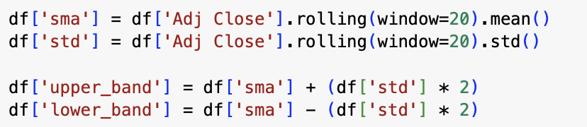
The Bollinger Bands is a technical indicator that’s plotted two commonplace deviations, each positively and negatively, away from a easy shifting common (SMA) of a safety’s worth. On this backtest, we’re going to use the standard configuration that’s 2 commonplace deviations +/- from a 20-day easy shifting common.
To calculate this in Python, we are going to create two new columns in df: one for the straightforward shifting common and the opposite for the usual deviation. In each circumstances, we’re going to use the .rolling() perform from pandas. The one distinction lies within the methodology appended on the finish: .imply() for computing the SMA and .std() for calculating the usual deviation.

Now the one factor left is to create one other two columns in df for the higher and decrease band. Within the higher band column, we are going to sum two commonplace deviations to the SMA, and within the decrease band, we are going to relaxation to straightforward deviations from the SMA.
Now that we’ve calculated the Bollinger Bands, we are able to start doing the backtest.
Calculating the returns of the technique
The technique we’re going to backtest is fairly straightforward:
- We purchase when the closing worth is underneath the decrease Bollinger Band
- We promote the value crosses above the higher Bollinger Band
To be able to do that, we’re going to create a brand new empty column known as ‘place’. Then, ranging from the twentieth index (as a result of we select the 20-day SMA), we are going to assign a 1 worth to the row within the ‘place’ column when the adjusted shut is beneath the worth within the decrease band. In any other case, it assigns a price of 0.
To calculate the promote sign we are going to use the identical perform. Ranging from the twentieth index, we are going to assign a price of -1 to the row within the ‘place’ column if the adjusted shut is above the higher band. If not, it retains the earlier worth from the ‘place’ column. All of that is carried out utilizing the np.the place() perform from numpy.
Final, we create one other column to calculate the day by day returns of the technique. To do that, we are going to multiply the day by day change within the safety by the lagged values within the ‘place’ columns(shifted by 1), after which add 1 to the outcome.

As soon as we did this, we efficiently calculated the returns of the buying and selling technique.
Plotting the outcomes of the technique
Now, the one factor left to do is plot the returns to see the strategy’s equity curve.
We’ll create one final new column known as ‘cumulative returns’ in df the place we are going to calculate the cumulative returns of the ‘returns’ column utilizing the .cumprod() methodology.
Lastly, we are going to generate a plot showcasing the “cumulative returns” column. Using the .plot() perform, we create the plot with figsize=(11,7) to specify the size of the determine. The title of the plot is about as “Fairness Curve” utilizing title=’Fairness Curve’. This visible illustration portrays the buying and selling technique’s efficiency over time, offering insights into the evolution of cumulative returns. By invoking plt.present(), the plot is displayed on the display for commentary.

The Bollinger Band buying and selling technique compounded cash at a 2.65% per 12 months whereas it was solely invested 10.6% of the time. Please needless to say the aim of the article is to point out how you should use Python. The technique itself is just for informational functions.
How you can backtest a Bollinger Band buying and selling technique in Python – conclusion
To sum up, at the moment we explored the method of backtesting a Bollinger Band buying and selling technique utilizing Python. The technique might not have had a stellar efficiency, however with this information, you possibly can confidently discover and refine your individual buying and selling concepts, using Bollinger Bands as a robust device in your decision-making course of.
[ad_2]
Source link